A Mathematical Introduction to Computer Vision for the Application of Multi Camera Tracking
This is a brief introduction to the mathematics behind a multi-camera person-tracking pipeline I have been working on whereby twelve fixed, unsynchronised camera feeds of the same factory floor are turned into one coherent notion of “person A was standing here, doing this, at this time,” with an optional full 3D body-pose reconstruction on top. Every section below is one component of that pipeline - the pinhole camera model, calibration by direct linear transform, appearance-based re-identification, Kalman-filter tracking, multi-view triangulation, and the diagnostics used to sanity-check all of it.
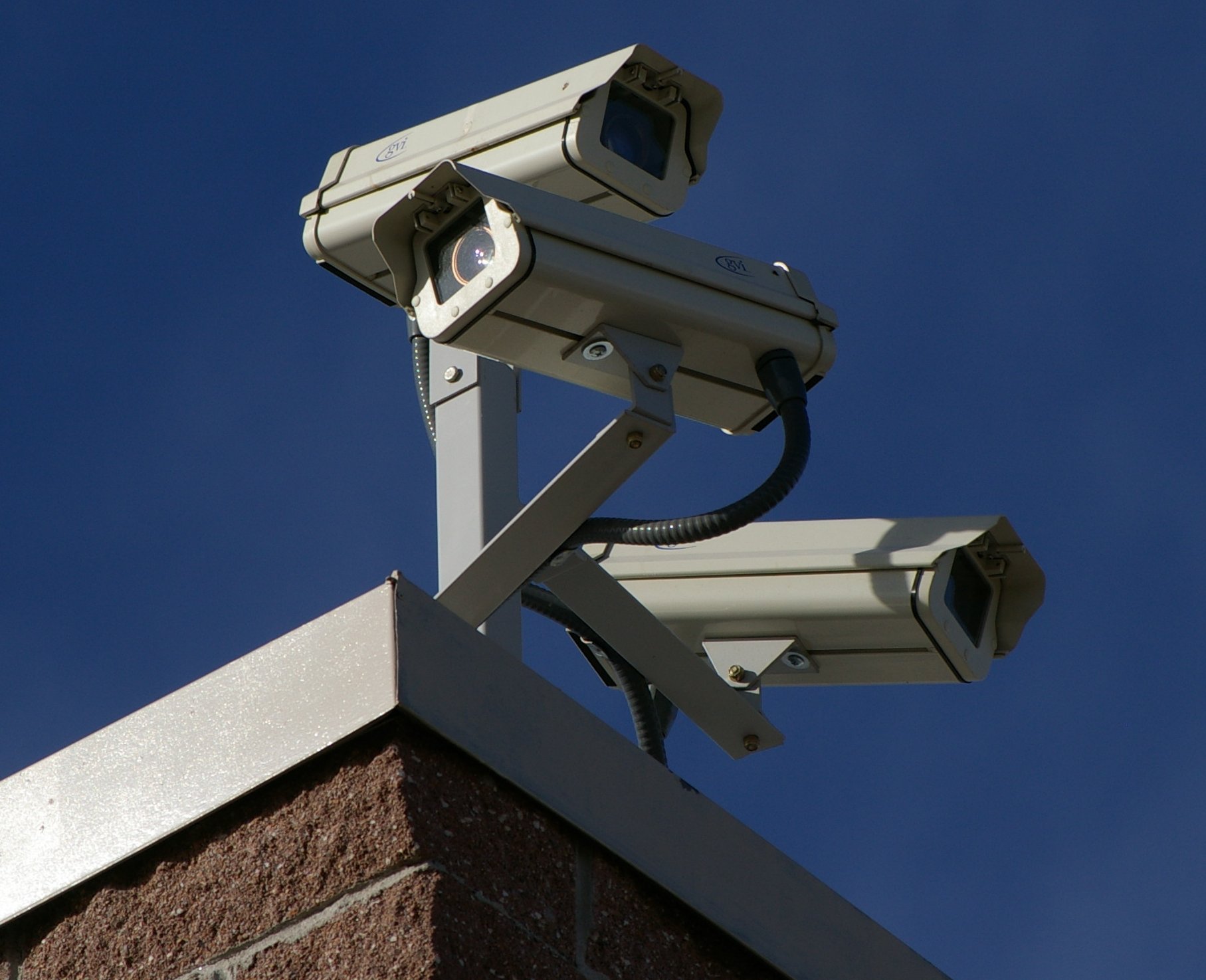
The pinhole camera model
Let a 3D Euclidean world point be
\[ \vect{X}_w = \begin{bmatrix} X & Y & Z \end{bmatrix}^{\top} \in \R^3, \qquad \homog{X} = \begin{bmatrix} X & Y & Z & 1 \end{bmatrix}^{\top} \in \mathbb{P}^3, \]
and let an image point be
\[ \vect{x} = \begin{bmatrix} u & v \end{bmatrix}^{\top} \in \R^2, \qquad \homog{x} = \begin{bmatrix} u & v & 1 \end{bmatrix}^{\top} \in \mathbb{P}^2, \]
where \( \mathbb{P}^n \) indicates a projective space in \(n\) dimensions, represented by an \((n{+}1)\)-valued vector.
Homogeneous coordinates are equivalence classes:
\[ \homog{x} \sim \lambda \homog{x}, \qquad \homog{X} \sim \mu \homog{X}, \qquad \lambda,\mu \in \R. \]
A projected point is therefore represented by all non-zero scalar multiples of that vector. This is the reason camera projection matrices, homographies, and DLT solutions are defined only up to an arbitrary scale factor.
The world-to-camera transform is
\[ \vect{X}_c = R\vect{X}_w + t = R(\vect{X}_w-\vect{C}), \qquad R\in SO(3), \qquad t=-R\vect{C}, \]
where \(R\) is a rotation, \(t\) is a translation, and \(\vect{C}\) is the camera centre in world coordinates. The intrinsic calibration matrix is
\[ K = \begin{bmatrix} f_x & s & c_x\\ 0 & f_y & c_y\\ 0 & 0 & 1 \end{bmatrix}, \]
where \(f_x,f_y\) are focal lengths in pixel units, \(s\) is skew, and \((c_x,c_y)\) is the principal point. The full pinhole projection matrix is therefore
\[ P = K\begin{bmatrix}R \mid t\end{bmatrix}\in\R^{3\times4}. \]
Since \(P\) has 12 scalar entries but is invariant under multiplication by any non-zero scalar, it has \(12-1=11\) projective degrees of freedom. The same count is recovered by inspection as 5 intrinsic degrees of freedom, 3 rotational degrees of freedom, and 3 translational degrees of freedom.
The pinhole projection equation is
\[ w \begin{bmatrix} u\\v\\1 \end{bmatrix} = P \begin{bmatrix} X\\Y\\Z\\1 \end{bmatrix} = \begin{bmatrix} \vect{p}_1^{\top}\homog{X}\\ \vect{p}_2^{\top}\homog{X}\\ \vect{p}_3^{\top}\homog{X} \end{bmatrix}, \]
where \(\vect{p}_i^{\top}\) denotes row \(i\) of \(P\), and \(w = \vect{p}_3^{\top}\homog{X}\) is the projective depth. Dehomogenising - dividing by the projective depth \(w\) - gives
\[ u = \frac{\vect{p}_1^{\top}\homog{X}}{\vect{p}_3^{\top}\homog{X}}, \qquad v = \frac{\vect{p}_2^{\top}\homog{X}}{\vect{p}_3^{\top}\homog{X}}. \]
The sign of \(w\) is physically meaningful after a camera orientation has been chosen such that for a valid calibration convention, points visible in front of the camera should have positive depth.
Camera calibration
Ground-plane homography
For a ground-plane point \(\homog{X}_{\pi}=[X,Y,1]^{\top}\), the planar homography satisfies
\[ s\homog{x}=H\homog{X}_{\pi}, \qquad H= \begin{bmatrix} h_1&h_2&h_3\\ h_4&h_5&h_6\\ h_7&h_8&h_9 \end{bmatrix}. \]
Let
\[ H\homog{X}_{\pi} = \begin{bmatrix} h_1X+h_2Y+h_3\\ h_4X+h_5Y+h_6\\ h_7X+h_8Y+h_9 \end{bmatrix} = \begin{bmatrix} x'\\y'\\w' \end{bmatrix}. \]
The inhomogeneous equations \(u=x'/w'\) and \(v=y'/w'\) imply
\[ u(h_7X+h_8Y+h_9)-(h_1X+h_2Y+h_3)=0, \] \[ v(h_7X+h_8Y+h_9)-(h_4X+h_5Y+h_6)=0. \]
Equivalently, one correspondence contributes two rows to \(A\vect{h}=0\):
\[ \begin{bmatrix} -X & -Y & -1 & 0 & 0 & 0 & uX & uY & u\\ 0 & 0 & 0 & -X & -Y & -1 & vX & vY & v \end{bmatrix} \begin{bmatrix} h_1\\h_2\\h_3\\h_4\\h_5\\h_6\\h_7\\h_8\\h_9 \end{bmatrix} = \vect{0}. \]
Stacking \(N\) correspondences gives \(A\in\R^{2N\times9}\). The Direct Linear Transform (DLT) estimate is the right singular vector associated with the smallest singular value:
\[ \vect{h}^{\star} = \argmin_{\|\vect{h}\|_2=1}\|A\vect{h}\|_2^2. \]
Since \(H\) has 9 entries but one arbitrary scale, it has 8 degrees of freedom, and four non-collinear correspondences are the algebraic minimum needed to produce it.
Plain least squares assumes every correspondence is reliable. The RANSAC algorithm instead samples minimal four-point subsets, estimates candidate homographies, and scores each candidate using the reprojection residual
\[ e_i(H)= \left\| \vect{x}_i- \pi\!\left(H\homog{X}_{\pi,i}\right) \right\|_2, \qquad \pi([a,b,c]^{\top})=[a/c,b/c]^{\top}. \]
The inlier set is \( \mathcal{I}(H)=\{i:e_i(H)<\tau_{\mathrm{ransac}}\} \), and the final estimate is refit on the largest consistent inlier set. It should be noted that the inlier set is calculated via N iterations of a random sample consensus to the end of reducing bias.
World ↔ map-pixel coordinates
Let \((X,Y)\) denote metric floor coordinates and let \((m,n)\) denote pixel coordinates on the top-down site map. A general affine conversion is
\[ \begin{bmatrix} m\\n\\1 \end{bmatrix} = A_{\mathrm{map}} \begin{bmatrix} X\\Y\\1 \end{bmatrix}, \qquad A_{\mathrm{map}}= \begin{bmatrix} a_{11} & a_{12} & a_{13}\\ a_{21} & a_{22} & a_{23}\\ 0 & 0 & 1 \end{bmatrix}. \]
For an axis-aligned map with separate horizontal and vertical scales, this reduces to
\[ m=s_xX+m_0, \qquad n=-s_yY+n_0. \]
The negative sign is normally present because image coordinates increase downwards, while a metric \(Y\)-axis is usually chosen to increase upwards on the floor plan.
This conversion is kept separate from the camera homography because it is not a camera calibration. The homography estimates the physical map from camera pixels to the metric ground plane, whereas \(A_{\mathrm{map}}\) is only a display transform from the metric ground plane to top-down image pixels. Changing the drawing, cropping the floor image, or changing the pixel scale should not require re-estimating any camera geometry.
Full 3D calibration via the Direct Linear Transform
For a full 3D correspondence \(\homog{X}=[X,Y,Z,1]^{\top}\) and image point \(\homog{x}=[u,v,1]^{\top}\),
\[ s\homog{x}=P\homog{X}. \]
Writing the rows of \(P\) as \( P= \begin{bmatrix} \vect{p}_1^{\top}\\ \vect{p}_2^{\top}\\ \vect{p}_3^{\top} \end{bmatrix} \), the two independent equations are
\[ u(\vect{p}_3^{\top}\homog{X})-\vect{p}_1^{\top}\homog{X}=0, \qquad v(\vect{p}_3^{\top}\homog{X})-\vect{p}_2^{\top}\homog{X}=0. \]
If the unknown vector is \( \vect{p}= \begin{bmatrix} \vect{p}_1\\\vect{p}_2\\\vect{p}_3 \end{bmatrix} \in\R^{12} \), one correspondence contributes
\[ \begin{bmatrix} \homog{X}^{\top} & \vect{0}^{\top} & -u\homog{X}^{\top}\\ \vect{0}^{\top} & \homog{X}^{\top} & -v\homog{X}^{\top} \end{bmatrix} \vect{p} = \vect{0}, \]
up to an arbitrary row sign convention. Stacking \(N\) points gives \(A\vect{p}=0\), with \(A\in\R^{2N\times12}\), and the DLT estimate is
\[ \vect{p}^{\star} = \argmin_{\|\vect{p}\|_2=1}\|A\vect{p}\|_2^2. \]
Because \(P\) has 11 degrees of freedom, six correspondences give twelve scalar equations and are the algebraic minimum, provided the 3D points are not all coplanar and are otherwise in a non-degenerate configuration.
If all calibration points lie on one plane, the full \(P\) cannot be identified. For example, if \(Z=0\), then
\[ P \begin{bmatrix} X\\Y\\0\\1 \end{bmatrix} = \begin{bmatrix} \vect{p}_1 & \vect{p}_2 & \vect{p}_4 \end{bmatrix} \begin{bmatrix} X\\Y\\1 \end{bmatrix}, \]
so only the three columns \(\vect{p}_1,\vect{p}_2,\vect{p}_4\) are observed. The third column, which controls how image position changes with height, does not enter the equations. Points at two or more distinct heights are therefore required for a non-degenerate 3D calibration.
Decomposing \(P\) into \(K\), \(R\), \(t\)
Let \( P= \begin{bmatrix} M \mid \vect{p}_4 \end{bmatrix} \), \(M\in\R^{3\times3}\). Since \(P=K[R\mid t]\), the left block satisfies \(M=KR\). The appropriate factorisation is RQ decomposition, where \(K\) is upper triangular and \(R\) is orthonormal - QR decomposition would give an orthonormal factor followed by an upper triangular factor, which is the reverse of the camera model. After RQ, the diagonal sign ambiguity is removed with
\[ D=\diag(\operatorname{sign}(K_{11}), \operatorname{sign}(K_{22}), \operatorname{sign}(K_{33})), \] \[ K\leftarrow KD, \qquad R\leftarrow DR, \qquad K\leftarrow K/K_{33}. \]
If \(\det(R)<0\), an additional global sign correction is required to return \(R\) to \(SO(3)\).
The camera centre is the right null vector of \(P\): \( P\homog{C}=\vect{0} \). If \(\homog{C}=[C_x,C_y,C_z,C_w]^{\top}\), then
\[ \vect{C}= \frac{1}{C_w} \begin{bmatrix} C_x\\C_y\\C_z \end{bmatrix}, \qquad t=-R\vect{C}. \]
The SVD solution to \(A\vect{p}=0\) is defined only up to sign: both \(P\) and \(-P\) produce the same image points after dehomogenisation. The sign is not harmless during decomposition, because it can produce negative focal lengths, an invalid rotation determinant, or a calibration in which visible world points have negative depth. A sign check is therefore
\[ d_i=\vect{p}_3^{\top}\homog{X}_i, \qquad \text{choose the sign of }P\text{ such that } \median_i(d_i)>0. \]
If a reconstruction appears mirrored, has \(K_{11}<0\), \(K_{22}<0\), or places calibration points behind the camera, the first debugging step is to inspect the depth signs \(d_i\) and flip the global sign of \(P\) if needed.
Calibration quality diagnostics
For either \(H\) or \(P\), the reprojection residual is \( \vect{r}_i= \vect{x}_i-\pi(A\homog{X}_i) \), where \(A=H\) for planar calibration and \(A=P\) for full 3D calibration. The root-mean-square reprojection error is
\[ \mathrm{RMSE} = \sqrt{\frac{1}{N}\sum_{i=1}^{N}\|\vect{r}_i\|_2^2}. \]
A good RMSE is on the order of the point-picking uncertainty. If a human click is expected to be accurate to \(\sigma_{\mathrm{click}}\) pixels, then a natural working threshold is a small multiple of that uncertainty, typically \( \tau_{\mathrm{rmse}}\approx 2\sigma_{\mathrm{click}} \) to \( 3\sigma_{\mathrm{click}} \). Errors well above this level indicate incorrect correspondences, a poor point configuration, unmodelled distortion, or a mismatch between the assumed world coordinate system and the clicked image points.
A single scalar RMSE is insufficient. Residual vectors \( \vect{r}_i = \begin{bmatrix} r_{u,i}\\r_{v,i} \end{bmatrix} \) should also be inspected spatially. Randomly oriented, zero-mean residuals suggest noise-limited calibration. Residuals with a coherent direction suggest an axis/sign error or an incorrect map transform. Residual magnitudes that increase radially from the principal point suggest unmodelled lens distortion. A simple distortion signature is the correlation
\[ \rho_{\mathrm{radial}} = \operatorname{corr}\!\left( \|\vect{r}_i\|_2, \left\|\vect{x}_i-\vect{c}\right\|_2 \right), \]
where \(\vect{c}=(c_x,c_y)^{\top}\). Values near zero are preferred; a large positive value indicates that a distortion model should be added.
For RANSAC homography fitting, the inlier ratio is \( \rho_{\mathrm{inlier}} = |\mathcal{I}|/N \). A high ratio means most correspondences agree with one planar model; a low ratio means the data contain many outliers or the assumed plane is wrong.
For SVD-based fits, let the singular values of \(A\) be \( \sigma_1\geq\sigma_2\geq\cdots\geq\sigma_n \). The solution is the right singular vector associated with \(\sigma_n\). A useful degeneracy score is \( g=\sigma_{n-1}/\sigma_n \). A large gap means the null direction is well separated; a gap close to one means the two smallest singular directions are nearly indistinguishable, so small annotation noise can cause a large change in the fitted model.
Perturbation testing quantifies the stability so that for trial \(j\), one will perturb clicked points by \( \vect{x}_i^{(j)} = \vect{x}_i+\epsilon_i^{(j)} \), \( \epsilon_i^{(j)}\sim\mathcal{N}(\vect{0}, \sigma_{\mathrm{click}}^2I) \), refit the calibration, and measure the spread of the resulting projections or recovered world points. A stable calibration has perturbation spread below the spatial tolerance required by the tracker; an unstable calibration needs more points, a wider spatial spread of points, or points at additional heights. Homographies are especially sensitive when points are nearly collinear or when the calibrated region is extrapolated beyond the convex hull of the clicked points.
SIFT keypoint detection
Calibration needs a keypoint-assisted point-picking UI because clicking precise, stable correspondences by eye is unreliable; SIFT keypoints give candidate click targets that are stable across both image location and image scale. The scale-space image is
\[ L(x,y,\sigma)=G(x,y,\sigma)*I(x,y), \qquad G(x,y,\sigma)= \frac{1}{2\pi\sigma^2} \exp\!\left( -\frac{x^2+y^2}{2\sigma^2} \right), \]
a Gaussian smoothing kernel. SIFT uses the Difference of Gaussians
\[ D(x,y,\sigma) = L(x,y,k\sigma)-L(x,y,\sigma), \]
which approximates the scale-normalised Laplacian of Gaussian:
\[ D(x,y,\sigma) \approx (k-1)\sigma^2\nabla^2 L(x,y,\sigma). \]
Candidate keypoints are local extrema of \(D\) in a \(3\times3\times3\) neighbourhood: eight neighbours in the same scale, nine in the scale above, and nine in the scale below. The image pyramid is formed by repeatedly smoothing an octave with increasing \(\sigma\), then downsampling to start the next octave. Points that survive this process are stable across both image location and image scale, which is why they are useful as click targets for calibration.
Object detection and pose estimation (YOLO)
Object detection
For a predicted box \(B_i\), class \(c_i\), and confidence \(q_i\), confidence thresholding is the decision rule \( \mathcal{D} = \{i:q_i\geq \tau_{\mathrm{det}}\} \). If explicit non-maximum suppression is required, boxes are sorted by confidence and lower-scoring boxes are suppressed when
\[ \IoU(B_i,B_j) = \frac{|B_i\cap B_j|}{|B_i\cup B_j|} > \tau_{\mathrm{nms}}. \]
An end-to-end (“end2end”) detector head is trained to output already de-duplicated detections directly, without a separate NMS step. Applying NMS when it is not needed can suppress valid close-together people; failing to apply NMS when it is needed can produce duplicate tracks from one person - so knowing which regime a given model head assumes is not optional.
Pose estimation
For a detector output indexed by \(i\), write \(d_i=(B_i,c_i,q_i)\), where \(B_i=(x_i,y_i,w_i,h_i)\) is the predicted bounding box, \(c_i\) is the class label, and \(q_i\in[0,1]\) is the detection confidence. In models with separate objectness and class probabilities, this confidence is commonly
\[ q_i = p(\mathrm{object}\mid B_i)\, p(c_i\mid B_i,\mathrm{object}). \]
A confidence threshold keeps detections satisfying \(q_i\geq \tau_{\mathrm{det}}\).
The pose model runs on a cropped detection rather than the full frame, since a tight crop gives the pose network a consistent scale and removes irrelevant background/other people from consideration. For a crop with top-left coordinate \((x_0,y_0)\), width \(W\), and height \(H\), a pose head returns COCO’s 17 keypoints,
\[ \mathcal{K} = \{(x_k,y_k,\alpha_k)\}_{k=1}^{17}, \]
where \(\alpha_k\in[0,1]\) is the keypoint confidence. If the model predicts normalised crop coordinates \((\xi_k,\eta_k)\), then the corresponding full-frame point is
\[ x_k=x_0+W\xi_k, \qquad y_k=y_0+H\eta_k. \]
If more than one pose is returned for the same crop, a simple selection score is
\[ S_{\mathrm{pose}} = q_{\mathrm{box}} \left( \frac{1}{17}\sum_{k=1}^{17}\alpha_k \right), \]
and the pose with the largest \(S_{\mathrm{pose}}\) is retained.
Re-identification (ReID) and cross-camera fusion
Appearance embeddings
A ReID network maps a crop \(I_i\) to an embedding \( \vect{f}_i=\phi_{\theta}(I_i)\in\R^d \). Embeddings are normally \(L^2\)-normalised: \( \vect{e}_i=\vect{f}_i/\|\vect{f}_i\|_2 \). The cosine similarity between two crops is then
\[ s_{ij} = \cos(\vect{e}_i,\vect{e}_j) = \frac{\vect{e}_i^{\top}\vect{e}_j}{\|\vect{e}_i\|_2\|\vect{e}_j\|_2} = \vect{e}_i^{\top}\vect{e}_j. \]
For unit vectors, squared Euclidean distance and cosine similarity are monotonically related:
\[ \|\vect{e}_i-\vect{e}_j\|_2^2 = 2-2\vect{e}_i^{\top}\vect{e}_j = 2(1-s_{ij}). \]
Cosine similarity is therefore scale-invariant: it compares the direction of appearance descriptors rather than their raw magnitude - which is what makes it preferable to a raw Euclidean distance here, since embedding magnitude is not a meaningful signal on its own.
Same-instant, cross-camera clustering
For detections \(i\) and \(j\) at the same frame, let \( \vect{g}_i=(X_i,Y_i)^{\top} \) be the projected ground-plane position and let \( \vect{e}_i\in\R^d \), \( \|\vect{e}_i\|_2=1 \), be the appearance embedding. Define \( \delta_{ij}=\|\vect{g}_i-\vect{g}_j\|_2 \) and \( s_{ij}=\vect{e}_i^{\top}\vect{e}_j \). A conservative same-instant merge rule is
\[ i\sim j \quad\Longleftrightarrow\quad c_i\neq c_j,\quad \delta_{ij}\leq r_{\mathrm{pos}}, \quad s_{ij}\geq \tau_{\mathrm{app}}, \]
where \(c_i\) is the camera index, \(r_{\mathrm{pos}}\) is the maximum acceptable cross-camera ground-plane separation, and \(\tau_{\mathrm{app}}\) is the minimum cosine similarity. Proximity alone is not sufficient because two different people can stand close together; appearance alone is not sufficient because two different cameras' lighting/angle can make the same person look different, or two different people look similar. A softer fused gate combines both into one score:
\[ D_{ij}^2 = \left(\frac{\delta_{ij}}{\sigma_{\mathrm{pos}}}\right)^2 + \left(\frac{1-s_{ij}}{\sigma_{\mathrm{app}}}\right)^2, \qquad \text{merge if } D_{ij}^2\leq \tau_{\mathrm{fuse}}^2. \]
The clusters are the connected components of this pairwise relation. For a cluster \(\mathcal{C}\), the fused ground position and embedding are
\[ \bar{\vect{g}} = \frac{\sum_{i\in\mathcal{C}}w_i\vect{g}_i}{\sum_{i\in\mathcal{C}}w_i}, \qquad \bar{\vect{e}} = \frac{\sum_{i\in\mathcal{C}}w_i\vect{e}_i}{\left\|\sum_{i\in\mathcal{C}}w_i\vect{e}_i\right\|_2}, \]
where \(w_i\) can be chosen from detection confidence, pose confidence, or a camera-quality weight.
Same-identity vs. different-identity similarity distributions
Given labelled or trusted identity assignments \(y_i\), define
\[
\mathcal{S}_{+} = \{s_{ij}:y_i=y_j,\ i
For a threshold \(\tau\), the false split and false merge rates are
\[
\mathrm{FSR}(\tau) = \Pr(s<\tau\mid \mathrm{same}),
\qquad
\mathrm{FMR}(\tau) = \Pr(s\geq\tau\mid \mathrm{different}).
\]
Plotting the two cosine-similarity distributions directly is a more actionable diagnostic than an embedding-space visualisation, because it answers the operational question head-on: if the empirical histograms of \(\mathcal{S}_{+}\) and \(\mathcal{S}_{-}\) overlap strongly, no single threshold can simultaneously make both the false-split and false-merge rates small, and no amount of retuning \(\tau_{\mathrm{app}}\) will fix that - the embedding itself needs to improve.
Use \(\vect{x}_t\) for the tracker state and \(\Sigma_t\) for its covariance, to avoid overloading \(P\), which already denotes the camera projection matrix. A constant-velocity state is
\[
\vect{x}_t= \begin{bmatrix} X_t\\Y_t\\\dot{X}_t\\\dot{Y}_t \end{bmatrix}.
\]
For elapsed time \(\Delta t\),
\[
F(\Delta t)=
\begin{bmatrix}
1&0&\Delta t&0\\
0&1&0&\Delta t\\
0&0&1&0\\
0&0&0&1
\end{bmatrix}.
\]
Assuming white acceleration noise with spectral scale \(q\), the process noise is
\[
Q(\Delta t)=q
\begin{bmatrix}
\frac{\Delta t^4}{4}&0&\frac{\Delta t^3}{2}&0\\
0&\frac{\Delta t^4}{4}&0&\frac{\Delta t^3}{2}\\
\frac{\Delta t^3}{2}&0&\Delta t^2&0\\
0&\frac{\Delta t^3}{2}&0&\Delta t^2
\end{bmatrix}.
\]
The scale \(q\) can be tied to an assumed maximum acceleration or maximum speed, for example \(q\propto v_{\max}^2\), so that uncertainty expands faster when longer occlusions or faster motion must be tolerated.
The prediction step is
\[
\hat{\vect{x}}_{t|t-1}=F\hat{\vect{x}}_{t-1|t-1},
\qquad
\Sigma_{t|t-1} = F\Sigma_{t-1|t-1}F^{\top}+Q.
\]
Only position is measured directly, so the measurement model is
\[
\vect{z}_t=H\vect{x}_t+\vect{\eta}_t,
\qquad
H= \begin{bmatrix} 1&0&0&0\\ 0&1&0&0 \end{bmatrix},
\qquad
\vect{\eta}_t\sim\mathcal{N}(\vect{0},R_m).
\]
The innovation and innovation covariance are
\[
\vect{y}_t=\vect{z}_t-H\hat{\vect{x}}_{t|t-1},
\qquad
S_t=H\Sigma_{t|t-1}H^{\top}+R_m.
\]
The Kalman gain is \( K_t=\Sigma_{t|t-1}H^{\top}S_t^{-1} \), and the correction step is
\[
\hat{\vect{x}}_{t|t} = \hat{\vect{x}}_{t|t-1}+K_t\vect{y}_t,
\qquad
\Sigma_{t|t} = (I-K_tH)\Sigma_{t|t-1}(I-K_tH)^{\top} + K_tR_mK_t^{\top}.
\]
The covariance \(\Sigma_t\) is the tracker uncertainty. Its position block grows during prediction and shrinks after measurement correction. Velocity is not directly observed; it is inferred through repeated position measurements and the cross-covariance terms between position and velocity.
The innovation \(\vect{y}_t=\vect{z}_t-H\hat{\vect{x}}_{t|t-1}\) has covariance \(S_t=H\Sigma_{t|t-1}H^{\top}+R_m\). Here \(R_m\) is the measurement-noise covariance matrix, describing the uncertainty in the measured position \(\vect{z}_t\). Since the measurement contains only the two position coordinates, \(R_m\in\R^{2\times 2}\); a common choice is
\[
R_m= \begin{bmatrix} \sigma_x^2 & 0\\ 0 & \sigma_y^2 \end{bmatrix},
\]
reducing to \(R_m=\sigma_m^2 I_2\) if measurement uncertainty is assumed equal in both directions. Larger \(R_m\) means the tracker trusts the measurement less; smaller \(R_m\) means it trusts the measurement more.
Under the Kalman model, \(\vect{y}_t\sim \mathcal{N}(\vect{0},S_t)\). Whitening the innovation, \(\vect{y}'_t=S_t^{-1/2}\vect{y}_t\), gives the squared Mahalanobis distance:
\[
d_M^2(\vect{z}_t) = \vect{y}_t^{\top}S_t^{-1}\vect{y}_t.
\]
A candidate detection is accepted only if \( d_M^2(\vect{z}_t)\leq \chi^2_{k,\alpha} \), where \(k=2\) for a 2D position measurement. Common choices are \(\chi^2_{2,0.95}=5.991\) and \(\chi^2_{2,0.99}=9.210\).
This is the uncertainty-aware generalisation of a fixed-radius gate. A fixed radius treats every direction as equally uncertain, which is wrong whenever the tracker is more confident in one direction than another (for instance, along the direction of motion vs. across it). If \(\Sigma\) is isotropic, the Mahalanobis gate is circular and reduces to the fixed-radius case; if uncertainty is larger in one direction than another, the gate becomes an ellipse aligned with the eigenvectors of \(S_t\), exactly matching the predicted shape of the measurement uncertainty.
A single overwritten reference embedding per identity is not enough, because appearance changes with pose, viewpoint, illumination, and partial occlusion - a track that briefly turns side-on or walks into shadow would otherwise permanently corrupt its own reference. Instead, for identity \(k\), store a bounded memory bank
\[
\mathcal{B}_k=\{(\vect{e}_{k,\ell},\omega_{k,\ell})\}_{\ell=1}^{M_k},
\qquad
M_k\leq M_{\max}.
\]
Let \(\mathcal{E}_k=\{\vect{e}_{k,1},\ldots,\vect{e}_{k,L_k}\}\) be the stored appearance memory for track \(k\), with \(L_k\) stored embeddings, and let \(\vect{e}\) denote a candidate embedding. All embeddings are \(\ell_2\)-normalised, so the inner product \(\vect{e}^{\top}\vect{e}_{k,\ell}\) is the cosine similarity. The weights \(\omega_{k,\ell}\geq 0\) control how much influence each stored embedding has; they may be uniform, or set according to recency, detection confidence, pose quality, or visibility.
The appearance score of a candidate embedding can be the maximum or weighted-average similarity:
\[
S_{\max}(k,\vect{e}) = \max_{\ell} \vect{e}^{\top}\vect{e}_{k,\ell},
\qquad
S_{\mathrm{avg}}(k,\vect{e}) = \frac{\sum_{\ell}\omega_{k,\ell}\vect{e}^{\top}\vect{e}_{k,\ell}}{\sum_{\ell}\omega_{k,\ell}}.
\]
A candidate match then requires both gates to pass:
\[
d_M^2\leq \chi^2_{2,\alpha}
\qquad\text{and}\qquad
S(k,\vect{e})\geq\tau_{\mathrm{app}}.
\]
A confidence-weighted exponential update for a prototype embedding is
\[
\vect{m}_k^{+} = \frac{(1-\eta q)\vect{m}_k+\eta q\vect{e}}{\|(1-\eta q)\vect{m}_k+\eta q\vect{e}\|_2},
\]
where \(q\) is the detection or keypoint confidence and \(\eta\) is a learning rate. The Kalman/Mahalanobis gate and the appearance memory bank combine to accept or reject a candidate match: motion alone can be fooled by two people crossing paths, and appearance alone can be fooled by two similarly-dressed people; requiring both is what makes the combination robust to either failure mode individually.
A moving subject’s pose is not a fixed shape, so it has to be triangulated fresh per-frame rather than aggregated into one static mesh. For camera \(j\), let
\[
P_j= \begin{bmatrix} \vect{p}_{j1}^{\top}\\ \vect{p}_{j2}^{\top}\\ \vect{p}_{j3}^{\top} \end{bmatrix},
\qquad
\homog{x}_j=[u_j,v_j,1]^{\top}.
\]
The unknown 3D keypoint \(\homog{X}\) satisfies \(s_j\homog{x}_j=P_j\homog{X}\). Eliminating the unknown scale \(s_j\) gives the two linear equations
\[
u_j(\vect{p}_{j3}^{\top}\homog{X}) - \vect{p}_{j1}^{\top}\homog{X} =0,
\qquad
v_j(\vect{p}_{j3}^{\top}\homog{X}) - \vect{p}_{j2}^{\top}\homog{X} =0.
\]
Equivalently, camera \(j\) contributes
\[
\begin{bmatrix}
u_j\vect{p}_{j3}^{\top}-\vect{p}_{j1}^{\top}\\
v_j\vect{p}_{j3}^{\top}-\vect{p}_{j2}^{\top}
\end{bmatrix}
\homog{X}
=
\vect{0}.
\]
With \(m\) confident views, the stacked system is \(A\homog{X}=\vect{0}\), \(A\in\R^{2m\times4}\) - the same SVD/homogeneous-system approach as calibration, one level up: solving for a point instead of a matrix. The triangulated point is the right singular vector associated with the smallest singular value:
\[
\homog{X}^{\star} = \argmin_{\|\homog{X}\|_2=1} \|A\homog{X}\|_2^2.
\]
At least two views are required because one view supplies only two independent equations for a homogeneous 3D point. With keypoint confidences \(\alpha_j\), the weighted version is
\[
\homog{X}^{\star} = \argmin_{\|\homog{X}\|_2=1} \|WA\homog{X}\|_2^2,
\qquad
W=\diag(\sqrt{\alpha_1},\sqrt{\alpha_1},\ldots, \sqrt{\alpha_m},\sqrt{\alpha_m}).
\]
If fewer than two views exceed the keypoint-confidence threshold, the point is simply not triangulable for that frame.
DLT minimises algebraic error, but not true reprojection error - the two coincide only approximately. The geometrically meaningful objective is reprojection error. For a 3D point \(\vect{X}\) and camera \(j\), define
\[
\pi(P_j\homog{X}) = \begin{bmatrix} \dfrac{\vect{p}_{j1}^{\top}\homog{X}}{\vect{p}_{j3}^{\top}\homog{X}}\\[4pt] \dfrac{\vect{p}_{j2}^{\top}\homog{X}}{\vect{p}_{j3}^{\top}\homog{X}} \end{bmatrix}.
\]
The residual is \(\vect{r}_j(\vect{X}) = \vect{x}_j-\pi(P_j\homog{X})\), and the nonlinear least-squares objective is
\[
E(\vect{X}) = \frac{1}{2} \sum_{j=1}^{m} \alpha_j \left\| \vect{r}_j(\vect{X}) \right\|_2^2.
\]
At iteration \(k\), linearise \(\vect{r}(\vect{X}_k+\Delta) \approx \vect{r}(\vect{X}_k)+J_k\Delta\), where \(J_k\) is the Jacobian of all residuals with respect to \((X,Y,Z)\). Levenberg–Marquardt solves
\[
\left(J_k^{\top}WJ_k + \lambda_k\diag(J_k^{\top}WJ_k) \right)\Delta = - J_k^{\top}W\vect{r}(\vect{X}_k).
\]
When \(\lambda_k\) is small, this approaches the Gauss–Newton step \((J^{\top}WJ)\Delta=-J^{\top}W\vect{r}\), which is fast near the optimum - Levenberg–Marquardt is an interpolation between Gauss–Newton and gradient descent. When \(\lambda_k\) is large, the diagonal damping dominates and the update behaves more like a cautious gradient-descent step. If a trial update decreases \(E\), it is accepted and \(\lambda_k\) is reduced; if it increases \(E\), the update is rejected and \(\lambda_k\) is increased.
The DLT point is a good initialisation, and the reason LM converges quickly from it, because it already satisfies the multi-view projection constraints approximately, even though it optimises algebraic rather than Euclidean image error. In practice, “success” means LM converges to a lower-reprojection-error point near the DLT initialisation; if it doesn’t converge (or makes things worse), the pipeline falls back to the unrefined DLT point rather than accepting a divergent refinement.
Let \(\vect{z}_i\in\R^d\) be a high-dimensional embedding and \(\vect{y}_i\in\R^2\) its low-dimensional visualisation. t-SNE defines conditional neighbour probabilities in the original space:
\[
p_{j|i} = \frac{ \exp\!\left(-\|\vect{z}_i-\vect{z}_j\|_2^2/(2\sigma_i^2)\right) }{ \sum_{k\neq i} \exp\!\left(-\|\vect{z}_i-\vect{z}_k\|_2^2/(2\sigma_i^2)\right) },
\qquad
p_{i|i}=0.
\]
The bandwidth \(\sigma_i\) is chosen so that a target perplexity holds:
\[
\operatorname{Perp}(P_i) = 2^{H(P_i)},
\qquad
H(P_i) = -\sum_{j}p_{j|i}\log_2 p_{j|i},
\]
making perplexity an effective neighbourhood-size knob: roughly, how many neighbours each point is expected to have non-negligible weight on. The symmetric joint probability is \( p_{ij}= (p_{j|i}+p_{i|j})/(2N) \).
In the embedded space, t-SNE uses a heavier-tailed Student-\(t\) kernel instead of a Gaussian:
\[
q_{ij} = \frac{ (1+\|\vect{y}_i-\vect{y}_j\|_2^2)^{-1} }{ \sum_{k\neq l} (1+\|\vect{y}_k-\vect{y}_l\|_2^2)^{-1} },
\qquad
q_{ii}=0.
\]
The heavier tail gives points more room to spread out in 2D without being unfairly penalised for the “crowding” that comes from cramming a high-dimensional neighbourhood into two dimensions. The optimisation objective is the Kullback–Leibler divergence
\[
C = D_{\mathrm{KL}}(P\|Q) = \sum_{i\neq j} p_{ij}\log\frac{p_{ij}}{q_{ij}}.
\]
Because KL divergence is asymmetric, t-SNE penalises missing true neighbours strongly: if \(p_{ij}\) is large but \(q_{ij}\) is small, the cost is large, while the reverse case is cheap. This is why t-SNE is mainly a local-neighbourhood diagnostic - it is very good at telling you whether points that should be close together actually cluster together, and much less trustworthy about the meaning of distances between distant clusters.
UMAP constructs a weighted \(k\)-nearest-neighbour graph instead of t-SNE’s Gaussian probability model. For point \(i\), let \(\rho_i\) be the distance to its nearest neighbour and \(\sigma_i\) a local scale. The directed membership strength from \(i\) to \(j\) is
\[
p_{j|i} = \exp\!\left( -\frac{\max(0,d(\vect{z}_i,\vect{z}_j)-\rho_i)}{\sigma_i} \right).
\]
Directed memberships are symmetrised by fuzzy union: \( p_{ij} = p_{j|i}+p_{i|j}-p_{j|i}p_{i|j} \). In the low-dimensional embedding,
\[
q_{ij} = \frac{1}{1+a\|\vect{y}_i-\vect{y}_j\|_2^{2b}},
\]
where \(a\) and \(b\) are determined by a chosen minimum-distance parameter. The cross-entropy objective is
\[
C = \sum_{i
The attractive term preserves high-confidence neighbours, while the repulsive term discourages unrelated points from collapsing together. UMAP is generally taken to preserve more of the global structure between clusters than t-SNE, at some cost in how faithfully it represents fine local neighbourhood density - which is exactly why it’s worth running both t-SNE and UMAP on the same embeddings rather than picking one: agreement between two algorithms with different distortion biases is a much stronger signal than either one alone.
The same-identity/different-identity similarity distributions introduced under re-identification above are also a visualisation technique in their own right. For bins \([b_r,b_{r+1})\), the empirical histogram estimates are
\[
\hat{p}_{+}(r) = \frac{1}{|\mathcal{S}_{+}|} \sum_{s\in\mathcal{S}_{+}} \mathbf{1}\{b_r\leq s
A useful scalar separation diagnostic is
\[
\Delta_{\mu} = \frac{\mu_{+}-\mu_{-}}{\sqrt{\frac{1}{2}(\sigma_{+}^2+\sigma_{-}^2)}},
\]
where \((\mu_{+},\sigma_{+})\) and \((\mu_{-},\sigma_{-})\) are the empirical means and standard deviations of same-identity and different-identity similarities. Larger \(\Delta_{\mu}\) means cleaner threshold separation - effectively an effect-size measure for how separable the two populations are, independent of any one chosen threshold \(\tau\).
Most of the mathematics in this pipeline is written using vectors, matrices, linear systems, least-squares problems, covariance matrices, and matrix factorisations. This section collects the most commonly used linear algebra so that the sections above on camera calibration, ReID, Kalman filtering, and 3D triangulation can be read more easily on their own.
A vector is an ordered list of numbers. In this document, column vectors are written in bold:
\[
\vect{x} = \begin{bmatrix} x_1\\x_2\\ \vdots \\ x_n \end{bmatrix} \in \R^n.
\]
A matrix is a rectangular array of numbers:
\[
A = \begin{bmatrix} a_{11} & a_{12} & \cdots & a_{1n}\\ a_{21} & a_{22} & \cdots & a_{2n}\\ \vdots & \vdots & \ddots & \vdots\\ a_{m1} & a_{m2} & \cdots & a_{mn} \end{bmatrix} \in \R^{m\times n}.
\]
The entry \(a_{ij}\) is the element in row \(i\) and column \(j\). Matrix multiplication is defined by taking dot products between rows of the first matrix and columns of the second matrix:
\[
(AB)_{ij} = \sum_{k} A_{ik}B_{kj}.
\]
For \(A\in\R^{m\times n}\) and \(\vect{x}\in\R^n\), the product \(A\vect{x}\in\R^m\) is
\[
A\vect{x} = \begin{bmatrix} \vect{a}_1^{\top}\vect{x}\\ \vect{a}_2^{\top}\vect{x}\\ \vdots\\ \vect{a}_m^{\top}\vect{x} \end{bmatrix},
\]
where \(\vect{a}_i^{\top}\) is row \(i\) of \(A\). Geometrically, a matrix can represent a linear transformation: it can rotate, scale, shear, project, or mix coordinates - every projection, calibration, and rotation elsewhere in this document is one instance of this same operation.
The transpose changes rows into columns: \(A^{\top}_{ij}=A_{ji}\). For two vectors \(\vect{x},\vect{y}\in\R^n\), the dot product is
\[
\vect{x}^{\top}\vect{y} = \sum_{i=1}^{n}x_i y_i.
\]
The dot product measures alignment. If two vectors point in a similar direction, their dot product is large and positive. If they are orthogonal, their dot product is zero: \(\vect{x}^{\top}\vect{y}=0\). The Euclidean norm of a vector is
\[
\|\vect{x}\|_2 = \sqrt{\vect{x}^{\top}\vect{x}} = \sqrt{\sum_{i=1}^{n}x_i^2}.
\]
A unit vector satisfies \(\|\vect{x}\|_2=1\). This is important for ReID embeddings because, after \(\ell_2\) normalisation, cosine similarity becomes a simple dot product:
\[
\cos(\vect{x},\vect{y}) = \frac{\vect{x}^{\top}\vect{y}}{\|\vect{x}\|_2\|\vect{y}\|_2} = \vect{x}^{\top}\vect{y}
\qquad
\text{if } \|\vect{x}\|_2=\|\vect{y}\|_2=1.
\]
A linear system has the form \(A\vect{x}=\vect{b}\). If \(A\in\R^{n\times n}\) is square and invertible, the solution is \(\vect{x}=A^{-1}\vect{b}\), where the inverse satisfies \(A^{-1}A=AA^{-1}=I\). However, many systems in camera calibration and triangulation are not solved by explicitly forming an inverse. Instead, they are solved using numerically stable factorisations such as QR decomposition or singular value decomposition -
[Draft note: the source document was cut off here, mid-sentence, before it could finish explaining SVD/least-squares for the general linear-algebra section and whatever followed it. Everything above this point is transcribed in full from the source; nothing below has been written yet - paste the rest and I'll continue it rather than invent an ending.]
Temporal tracking
The Kalman filter motion model
Mahalanobis gating
Appearance memory bank
3D skeleton reconstruction
Multi-view triangulation via DLT
Levenberg–Marquardt refinement
Dimensionality reduction and diagnostics
t-SNE
UMAP
Cosine similarity histograms as a diagnostic visualisation
Common linear algebra used throughout the pipeline
Vectors and matrices
Transpose, dot product, and norms
Linear systems
Discussion